Sigur Rós has been my favorite band for the last decade, ever since one of my high school boyfriends lent me a copy of Takk…. On Tuesday I saw them perform at the Paramount Theatre in Seattle. The show was spectacular as usual, and it got me curious about my history of listening to Sigur Rós.
I’ve had a last.fm account since 2009, so a good chunk of that listening history is preserved. Using this tool I downloaded my data and set out to visualize a decade (ish) of listening to Sigur Rós.
First I’ll load the data (available in my GitHub repository) and R packages I need. I also created a custom color palette for some of the plots in this post based on the cover of Með suð í eyrum við spilum endalaust (possibly NSFW).
## Load packages
library("tidyverse")
library("lubridate")
library("knitr")

## Load data
plays <- read_csv("../data/karawho_lastfm.csv",
                  col_names = c("artist", "album", "track", "date"),
                  col_types = cols(date = col_date(format = "%d %b %Y %H:%M")))

## Set ggplot2 theme
theme_set(theme_minimal() +
          theme(axis.text = element_text(size = 14),
                axis.title = element_text(size = 16),
                legend.text = element_text(size = 14)))

## Color palette
msievse <- c("#547a9e" ,"#d5bfa8", "#aec2cb", "#93775f", "#a0a17f", "#73715c",
             "#dfddd1", "#7598ac", "#4f3e36", "#6f7269")
Unfortunately, there are some issues with this data. At the time of writing, my last.fm profile shows 57,757 total “scrobbles” (songs played), but using the online tool I got a dataset of 53,527. Over 2000 rows in the dataset have a date of 1970-01-01. This might be data that I imported to last.fm when I signed up, but it’s hard to say. I’ll leave this data in for plots that don’t have to do with dates and remove it otherwise.
Also, my monthly play counts have a few months with no scrobbles whatsoever:
## Make sure all months after I created my account are represented in the data
all_months <- plays %>% expand(year(date), month(date)) %>%
  filter(`year(date)` >= 2009)

plays %>%
  group_by(year(date), month(date)) %>%
  right_join(all_months) %>%
  tally() %>%
  mutate(month = as.Date(paste(`year(date)`, `month(date)`, "01",
                               sep = "-"))) %>%
  ggplot(aes(x = month, y = n)) +
  geom_line() +
  labs(x = "Month", y = "Scrobbles")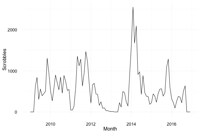
According to the data I didn’t listen to any music at all in April 2013 (among other months), but I actually saw Sigur Rós play in Santa Barbara on April 19th, 2013 and distinctly remember listening to them at home before and after the show. Perhaps scrobbling was broken and the tracks didn’t get saved.
The data is a little questionable and incomplete (since it only goes back to 2009), but it’s what I have, so let’s move on.
Top artists in my scrobbling history
Last.fm shows my most listened to artists as such:
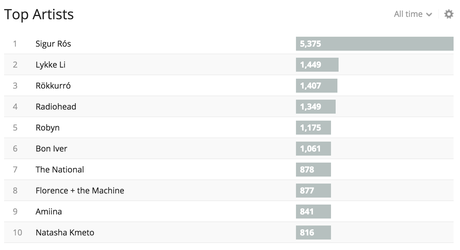
However, the plot from my data is slightly different.
top_10_artists <- plays %>%
  count(artist, sort = TRUE) %>%
  top_n(n = 10, wt = n)

ggplot(top_10_artists, aes(x = reorder(artist, n), y = n)) +
  geom_bar(stat = "identity") +
  geom_text(aes(label = n), position = position_dodge(0.9), hjust = 1.2,
            color = "white", size = 4) +
  labs(y = "Scrobbles", x = "") +
  coord_flip()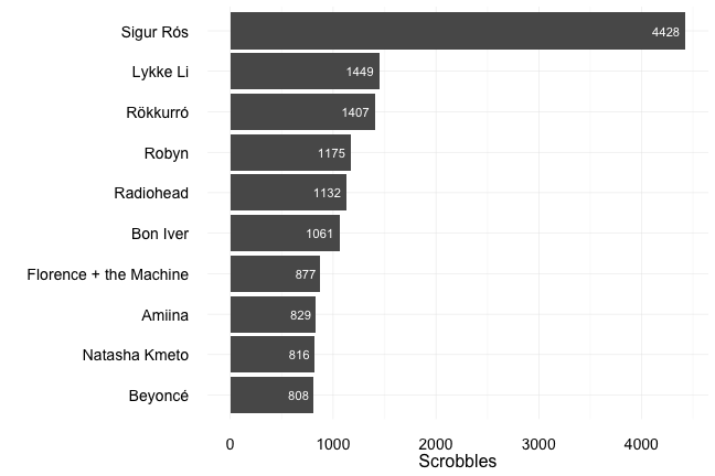
Inexplicably, The National is my seventh most listened to band on last.fm and doesn’t even appear in the top 10 in the data.
According to this I’ve listened to Sigur Rós 3.1 times as much as the next most listened to artist. What about compared to all other artists combined? In this case I’ll use a regex to match Sigur Rós because I have some Sigur Rós tracks that include collaborations with other artists.
plays %>%
  mutate(sr = ifelse(grepl("(s|S)igur\\s(r|R)(o|ó)s", artist),
                     "Sigur Rós", "other"),
         sr = factor(sr, levels = c("Sigur Rós", "other"))) %>%
  ggplot(aes(x = factor(1), fill = sr)) +
  geom_bar(width = 1) +
  coord_polar(theta = "y") +
  scale_fill_manual(values = msievse) +
  theme_void() +
  theme(legend.text = element_text(size = 14)) +
  labs(title = "Scrobbles")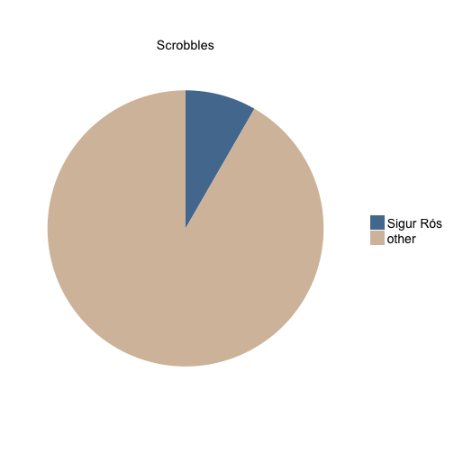
Sigur Rós makes up a total of 9 percent of my listening history. It’s definitely my most listened to band overall, but how often is it the top in a given year or month?
## Remove data with messed up year
plays_clean <- filter(plays, year(date) >= 2009)

plays_clean %>%
  group_by(year(date), artist) %>%
  tally() %>%
  top_n(1, wt = n) %>%
  rename(year = `year(date)`) %>%
kable()| year | artist | n |
|---|---|---|
| 2009 | Sigur Rós | 734 |
| 2010 | Sigur Rós | 911 |
| 2011 | Sigur Rós | 1125 |
| 2012 | Sigur Rós | 384 |
| 2013 | Beyoncé | 346 |
| 2014 | Sigur Rós | 429 |
| 2015 | Natasha Kmeto | 589 |
| 2016 | Sigur Rós | 288 |
Sigur Rós is frequently, but not always, my most listened to band in a year. It’s a bit less common that I listen to them the most in a given month:
plays_clean %>%
  group_by(year(date), month(date), artist) %>%
  tally() %>%
  top_n(1, wt = n) %>%
  mutate(sr = ifelse(grepl("(s|S)igur\\s(r|R)(o|ó)s", artist),
                     "Sigur Rós", "other"),
         sr = factor(sr, levels = c("Sigur Rós", "other")),
         month = as.Date(paste(`year(date)`, `month(date)`, "01",
                               sep = "-")),
         w = days_in_month(month) - 7) %>%
  ggplot(aes(x = month, y = 1)) +
  geom_tile(aes(fill = sr, width = w)) +
  scale_fill_manual(values = msievse) +
  labs(title = "Top artist", x = "Month", y = "", fill = "") +
  theme(axis.text.y = element_blank(),
        legend.position = "top",
        panel.grid.major = element_blank(),
        panel.grid.minor = element_blank(),
        plot.title = element_text(size = 18))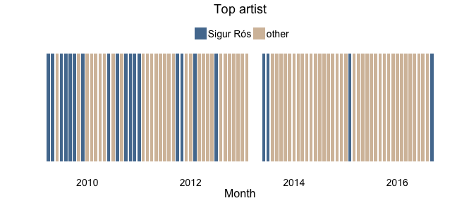
This fits with my impressions of my listening habits: I often get into a particular artist and listen to them a lot in a short period of time, but I listen to Sigur Rós pretty consistently. More on this shortly.
Sigur Rós listening habits over time
Here are my yearly and monthly scrobbles of Sigur Rós songs (note again the gaps that are visible when we look at the monthly data):
## Remove data from 1970
plays_clean_sr <- filter(plays_clean, grepl("(s|S)igur\\s(r|R)(o|ó)s", artist))

## Yearly
plays_clean_sr %>%
  group_by(year(date)) %>%
  tally() %>%
  ggplot(aes(x = `year(date)`, y = n)) +
  geom_line() +
  labs(x = "Year", y = "Scrobbles")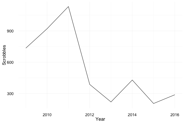
## Monthly
plays_clean_sr %>%
  group_by(year(date), month(date)) %>%
  right_join(all_months) %>%
  tally() %>%
  mutate(month = as.Date(paste(`year(date)`, `month(date)`, "01",
                               sep = "-"))) %>%
  ggplot(aes(x = month, y = n)) +
  geom_line() +
  annotate("rect",
           xmin = as.Date("2010-08-22"), xmax = as.Date("2011-05-20"),
           ymin = 0, ymax = 450, alpha = 0.2) +
  annotate("text", label = "Studied in Iceland", angle = 270,
           x = as.Date("2010-08-22"), y = 450, hjust = -0.05, vjust = -0.5) +
  labs(x = "Month", y = "Scrobbles")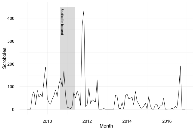
You can see the increasing listening counts around the start of my study abroad in Iceland, as well as when I was planning the study abroad in late 2009. I experienced a lot of re-entry culture shock when I came back and started the next school year. I had a hard time readjusting, which might be why I was listening to Sigur Rós so obsessively in the fall of 2011.
Getting back to the point I made above, here are the monthly scrobbles for my top 10 most listened to artists:
## Again, make sure we're not skipping months that claim to have no scrobbles
all_months_artists <- plays %>%
  filter(artist %in% top_10_artists$artist) %>%
  expand(year(date), month(date), artist) %>%
  filter(`year(date)` >= 2009)

plays_clean %>%
  filter(artist %in% top_10_artists$artist) %>%
  group_by(year(date), month(date), artist) %>%
  right_join(all_months_artists) %>%
  tally() %>%
  mutate(artist = factor(artist, levels = top_10_artists$artist)) %>%
  mutate(month = as.Date(paste(`year(date)`, `month(date)`, "01",
                               sep = "-"))) %>%
  ggplot(aes(x = month, y = n)) +
  geom_line() +
  facet_wrap(~ artist, ncol = 2) +
  theme(strip.text.x = element_text(size = 14)) +
  labs(x = "Month", y = "Scrobbles")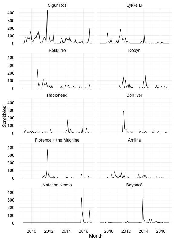
Indeed, some of my top artists definitely got onto the top 10 roster through short, intense periods of listening.
Top songs and albums
I looked at the cumulative play counts for my top 10 Sigur Rós albums. In this plot you can see when Inni, Valtari, and Kveikur were released in 2011, 2012, and 2013.
top_albums <- plays %>%
  filter(grepl("(s|S)igur\\s(r|R)(o|ó)s", artist) & year(date) >= 2009) %>%
  count(album, sort = TRUE) %>%
  top_n(n = 10, wt = n)

plays %>%
  filter(album %in% top_albums$album & year(date) >= 2009) %>%
  group_by(album) %>%
  mutate(count = n()) %>%
  ggplot(aes(x = date, color = reorder(album, 1 / count))) +
  geom_step(aes(len = count, y = ..y.. * len), stat = "ecdf", size = 1.5) +
  scale_color_manual(values = msievse) +
  labs(x = "Date", y = "Cumulative scrobbles", color = "Album")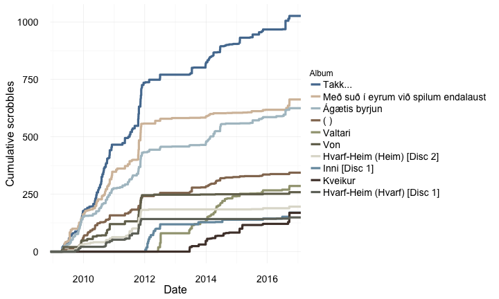
This is interesting to me. I don’t think of Takk… as my favorite album, yet I’ve clearly listened to it much more than any other. Then again, it was the first Sigur Rós album I heard so perhaps it shouldn’t be too surprising that I’ve listened to it the most.
I’m also a bit surprised that the data shows I’ve barely listened to Hvarf-Heim since 2012, because I quite like that album.
Finally, I looked at the Sigur Rós tracks I’ve listened to the most. This is a little tricky because I have live versions of many songs that appear on different albums. Should these all be counted separately or together? I chose to count them separately, in part because they often have different spellings in the data anyway (“Hafsól” vs. “Hafsol” or “Popplagið” vs. “Untitled 8”).
plays %>%
  filter(grepl("(s|S)igur\\s(r|R)(o|ó)s", artist) & year(date) >= 2009) %>%
  group_by(album, track) %>%
  tally(sort = TRUE) %>%
  ungroup() %>%
  top_n(n = 10) %>%
  ggplot(aes(x = reorder(track, n), y = n, fill = reorder(album, 1/n))) +
  geom_bar(stat = "identity") +
  scale_fill_manual(values = msievse) +
  geom_text(aes(label = n), position = position_dodge(0.9), hjust = 1.2,
            color = "white", size = 4) +
  labs(x = "Track", y = "Scrobbles", fill = "Album") +
  coord_flip()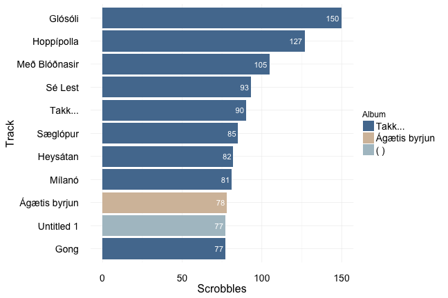
This is another place where my data disagrees with what last.fm shows online. They think my top Sigur Rós tracks are: Glósóli, Hoppípolla, Ágætis byrjun, Með Blóðnasir, Starálfur, Heysátan, Festival, Inní mér syngur vitleysingur, Sæglópur, and All alright.
So there you have it: more than you ever wanted to know about my Sigur Rós listening history.